Copyrights: Khoi Nguyen, My Nguyen, Khiet Dang, Bao Pham, Vy Huynh, Toi Vo, Lua Ngo, Huong Ha, 2023. License: This work is licensed under a Creative Commons Attribution 4.0 International License.
Abstract
Introduction: Early Alzheimer's disease (AD) diagnosis is critical to improving the success of new treatments in clinical trials, especially at the early mild cognitive impairment (EMCI) stage. This study aimed to tackle this problem by developing an accurate classification model for early AD detection at the EMCI stage based on magnetic resonance imaging (MRI).
Methods: This study developed the proposed classification model through a machine-learning pipeline with three main steps. First, features were extracted from MRI images using FreeSurfer. Second, the extracted features were filtered using principal component analysis (PCA), backward elimination (BE), and extreme gradient (XG)-Boost importance (XGBI), the efficiency of which was evaluated. Finally, the selected features were combined with cognitive scores (Mini Mental State Examination [MMSE] and Clinical Dementia Rating [CDR]) to create an XG-Boost three-class classifier: AD vs. EMCI vs. cognitively normal (CN).
Results: The MMSE and CDR had the highest importance weights, followed by the thickness of the left superior temporal sulcus and banks of the superior temporal lobe. Without feature selection, the model had the lowest accuracy of 69.0%. After feature selection and the addition of cognitive scores, the accuracy of the PCA, BE, and XGBI approaches improved to 74.0%, 90.9%, and 91.5%, respectively. The BE with tuning parameters model was chosen as the final model since it had the highest accuracy of 92.0%. The area under the receiver operating characteristic curve for the CN, AD, and EMCI classes were 0.98, 0.94, and 0.88, respectively.
Conclusion: Our proposed model shows promise in early AD diagnosis and can be fine-tuned in the future through testing on a multi-dataset.
Introduction
Alzheimer’s disease (AD) is the most common neurodegenerative disorder that greatly reduces patients’ quality of life and makes them utterly dependent on their caregivers1, 2. Prolonged medical treatment and care exert a substantial economic strain on patients and their families, potentially costing >1.1 trillion US dollars worldwide1. Unfortunately, once cognitive symptoms manifest, current medications cannot reverse disease progression due to the continued loss of neurons without replacement by cell division3, 4. Therefore, identifying patients at the early mild cognitive impairment (EMCI) stage is critical to improving the success of new treatments or interventions in clinical trials.
Several breakthrough approaches have attempted to predict AD at its preclinical stage, which could allow the application of medications to halt AD development from its onset3, 5, 6, 7, 8. About 80% of patients diagnosed with mild cognitive impairment (MCI) convert to AD within six years9. Recent studies have focused on this transitional phase to detect the preclinical AD stage, particularly EMCI5. One promising approach to detect EMCI is identifying brain morphological changes through neuroimaging data, such as magnetic resonance imaging (MRI).
Early AD detection using brain MRI data remains clinically challenging since the subtle changes during its transitional period cannot be assessed manually3. Automatic computation and artificial intelligence (AI) approaches such as deep learning (DL) or machine learning (ML) are required to identify brain structural features at the EMCI stage. Of numerous AI-assisted methods, DL has been broadly used because of its high performance, especially the convolutional neural network (CNN)5, 10. Kang et al. combined a 2D CNN with transfer learning to identify EMCI by processing a multi-modal dataset (MRI and diffusion tensor imaging data), achieving the highest accuracy of 94.2% for cognitively normal (CN) vs. EMCI patients5. In addition, Kolahkaj et al. built a DL architecture based on the BrainNet CNN model to detect EMCI, achieving high accuracies for binary classification: 0.96, 0.98, and 0.95 for NC/EMCI, NC/MCI, and EMCI/MCI, respectively11.
Despite its significant results, DL has several limitations that could hinder clinical applications. Firstly, DL models are prone to encounter overfitting due to the many parameters considered12. Secondly, analysts cannot provide a plausible explanation for the algorithm’s performance, which is called a black box. Therefore, to build an understandable prediction model, making the shift to ML for early AD detection is beneficial for neurologists and doctors.
While most ML studies have focused on binary classification, some have focused on multi-class classification. However, there is a growing need for a multi-class algorithm that can effectively distinguish the prodromal stage (EMCI) from the array of other stages (late MCI [LMCI], AD, and CN), enabling an early AD diagnosis. Moreover, it is important to note that existing multi-class ML models have low accuracies. In 2022, Techa et al. showed that a new model based on three CNN architectures (DenseNet196, VGG16, and ResNet50) achieved 89% accuracy in discriminating normal, very mild dementia, mild dementia, moderate dementia, and AD13. Alorf et al. implemented a Brain Connectivity-Based Convolutional Network in 2022, which provided 84.03% accuracy for six-class classification (AD, LMCI, MCI, EMCI, subjective memory complaints, and CN)14. Another major difficulty when identifying the initial AD stages is the subtle structural change in subjects with EMCI. EMCI is elusive and cannot be recognized by the diagnostic criteria for AD15. Furthermore, EMCI and MCI are highly heterogeneous since they can be easily mistaken for multiple pathological conditions, especially other neurodegenerative diseases16, 17. Therefore, EMCI classification requires further evaluation and approaches to optimize its efficiency.
One potential ML model to address the early AD detection challenge is extreme gradient boosting (XG-Boost). XG-Boost is a scalable tree-based ensemble learning implemented from the gradient boosting system. It introduces errors from the previous weak learner to the latter learner, improving its learning accuracy18. Since its results depend on many decision trees, XG-Boost shows high compatibility, competitive execution speed, and accuracy when applied to large data sets, making it suitable for clinical application19. While few studies have used XG-Boost for AD diagnosis, the preliminary results are promising. Ong et al. proposed an XG-Boost model to classify AD and CN subjects using the FreeSurfer library to extract insight features from MRI, achieving an area under the receiver operative characteristic (ROC) curve (AUC) of 91%20. Tuan et al. presented an XG-Boost model to classify AD and normal subjects based on the tissues segmented by a CNN and Gaussian mixture model21. Their highest accuracy was 89% when combined with a support vector machine (SVM) and CNN21. However, both models had several limitations, such as high computation cost and susceptibility to sample size and complexity. They also did not attempt to classify three classes. Therefore, future improvement is required to enhance the models’ accuracy and validity.
This study used XG-Boost for three-class classification, primarily focusing on distinguishing CN, EMCI, and AD. It also evaluated and optimized three feature selection methods—backward elimination, XG-Boost importance (XGBI), and principal component analysis (PCA)—to identify the most suitable method for the XG-Boost model. When combined with the Mini Mental State Examination (MMSE) and Clinical Dementia Rating (CDR) scores, our model achieved the highest accuracy of 92% for distinguishing AD, EMCI, and CN. Only three features overlapped between the BE and XGBI feature selection methods: MMSE, CDR, and left hippocampus volume. While these results showed that the model still depends on the cognitive symptoms of AD rather than its brain structural changes, our model has great potential as an assistive tool for AD diagnosis with high performance, especially when considering its multi-class classification.
Methods
Participants
This study obtained its data from the Alzheimer’s Disease Neuroimaging Initiative (ADNI) database (http://adni.loni.usc.edu)22. The ADNI was launched in 2003 as a public-private partnership led by Principal Investigator Michael W. Weiner, MD. Its primary goal has been to test whether serial MRI, positron emission tomography, biological markers, and clinical and neuropsychological assessments can be combined to measure MCI and EMCI progression22.
The data comprised 663 subjects who were equally grouped into three classes: CN, EMCI, and AD. Their demographic information is summarized in Table 1.
| CN | EMCI (n = 221) | AD (n = 221) | p | |
|---|---|---|---|---|
| Age | 75.28 ± 5.76 | 71.45 ± 7.23* | 75.4 ± 7.702 | < 0.0001 |
| Sex (M/F) | 120/101 | 118/103 | 120/101 | 0.9760 |
| MMSE Score | 29.06 ± 1.1 | 28.12 ± 1.66* | 22.8 ± 2.63* | < 0.0001 |
| CDR Score | 0.03 ± 0.11 | 0.47 ± 0.16* | 0.81 ± 0.32* | < 0.0001 |
| Education (Years) | 16.18 ± 3.88 | 16.09 ± 2.65 | 14.65 ± 4.35* | < 0.0001 |
| ApoE4 (+/-) | 157/64 | 82/139 | 58/163 | < 0.0001 |


| No. | Subject ID | Brain Segmentati-on Volume Without Ventricles | Left Entorhinal Cortex (temporal lobe) | White Surface Total Area in the left hemisphere | Banks of Superior Temporal Sulcus in the left hemisphere | ... | Number of Defect Holes in right hemispherical Surface Prior to fixin |
|---|---|---|---|---|---|---|---|
| 1 | 135_S_4598 | 1076438.0 | 285.0 | 84644.5 | 996.0 | ... | 17.0 |
| 2 | 099_S_4480 | 945976.0 | 310.0 | 76032.8 | 744.0 | ... | 33.0 |
| 3 | 099_S_2146 | 1138086.0 | 453.0 | 88770.5 | 1118.0 | ... | 46.0 |
| ... | ... | ... | ... | ... | ... | ... | ... |
| 662 | 082_S_1079 | 1131880.0 | 446.0 | 94008.6 | 1244.0 | ... | 73.0 |
| 663 | 130_S_5059 | 1160101.0 | 601.0 | 85947.9 | 862.0 | ... | 49.0 |
| * Where area in mm 2 , volume in mm 3 | |||||||


| Method | Backward Elimination (Approach 3) | XGBoost Importance (Approach 4) | PCA (Approach 5) |
|---|---|---|---|
| Number of features after selection | 29 | 228 | 71 |
| Type of features | Brain features and cognitive scores | Brain features and cognitive scores | PCA features |


| Approach | Class | Accuracy | Precision | Recall | F1 score |
|---|---|---|---|---|---|
| 1 | CN | 68.8 % | 64 % | 56 % | 60 % |
| EMCI | 64 % | 75 % | 69 % | ||
| AD | 79 % | 74 % | 77 % | ||
| 2 | CN | 86 % | 80 % | 97 % | 88 % |
| EMCI | 97 % | 71 % | 82 % | ||
| AD | 83 % | 98 % | 90 % | ||
| 3 | CN | 91.05 % | 89 % | 98 % | 93 % |
| EMCI | 95 % | 83 % | 89 % | ||
| AD | 91 % | 95 % | 93 % | ||
| 4 | CN | 90.9 % | 91 % | 98 % | 95 % |
| EMCI | 92 % | 79 % | 85 % | ||
| AD | 90 % | 96 % | 93 % | ||
| 5 | CN | 74 % | 68 % | 59 % | 63 % |
| EMCI | 75 % | 77 % | 76 % | ||
| AD | 78 % | 86 % | 82 % | ||
| 6 | CN | 92 % | 88 % | 97 % | 93 % |
| EMCI | 91 % | 85 % | 88 % | ||
| AD | 96 % | 94 % | 95 % |


Structural MRI data
The structural MRI scans used in this study were the T1-weighted magnetization prepared-rapid gradient echo scans from ADNI 1 and ADNI GO/2. Various MRI scanner models were used for MRI acquisition; details of the acquisition protocol for the MRI data can be found on the ADNI website (http://adni.loni.usc.edu)22.
Study design
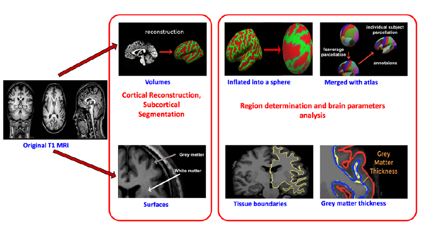
An overview of the study design is shown in Figure 1. Firstly, the MRI images were preprocessed with FreeSurfer to extract 358 features, including volumetric and thickness measurements. Three feature selection methods were used, and their efficiencies were compared. This step determined the optimal features from the 360 elements (FreeSurfer features, MMSE score, and CDR score). The data were divided into two sets with a ratio of 80% training to 20% testing using Python’s Scikit-learn library. Finally, the proposed models were evaluated using the performance metrics of accuracy, precision, recall, F1-score, and ROC curves with AUCs to identify the most efficient classification algorithm.
Feature extraction
Six hundred sixty-three MRI images were reconstructed and segmented using FreeSurfer (version 5.3; http://surfer.nmr.mgh.harvard.edu). This open-source software measures and visualizes the human brain’s functional, connective, and structural characteristics to extract brain structural features23. This software’s processing operations have two major stages (Figure 2).
Feature selection
Feature selection plays a significant role in ML and pattern recognition. Pearson’s product-moment correlation coefficient (r) was first applied to remove all linearly related features with a r > 0.9. The reason for using this method is that several features extracted by Freesurfer are sub-regions or different measurements of the same brain region. Therefore, including highly relevant features in a particular brain-diagnosed area is redundant from a neuroscience perspective. Moreover, highly correlated features may lead to overfitting, impacting model performance. Therefore, applying non-linear feature selection can improve model performance and reduce training time efficiently. The next step was performed with three feature selection methods to compare their efficiency.
PCA
PCA is a multivariate exploratory analysis approach that reduces the complexity of multidimensional data while preserving trends and key patterns24, 25. PCA was applied using Python’s Scikit-learn library with different numbers of principal components (PCs; 1–321) to determine the optimal set of features for the classification model. Then, in each model, the PCs were incrementally included in 10 PC increments to observe changes in accuracy with Python’s Matplotlib library.
BE
BE is a feature selection strategy that excludes characteristics strongly associated with the exposure without significantly influencing dependent variables or predicted outputs26, 27. BE was applied in five main steps: (i) select a significance level (SL) that is suitable for the model (SL = 0.05), (ii) calculate original least squares with Python’s Statsmodels library before determining the p-values of all features, (iii) compare the calculated p-value with the SL, (iv) remove features and predictors with a p-value greater than the SL, and (v) modify it to fit the model with the remaining variables.
XGBI
XG-Boost has the advantage of extracting importance scores for each feature in the predictive problem, enabling the determination of the highest importance score. The next step removes all unusable features with zero importance coefficients depending on their ranking. This action is repeatedly performed until stable accuracy and non-zero importance coefficients are achieved.
Six features selection approaches
This study investigated six approaches for feature selection. Feature selection was not applied in the first and second approaches. The first approach used all 358 features extracted by Freesurfer to train the model. The second approach added the two cognitive scores to the 358 Freesurfer features. The third approach used XGBI to filter the Freesurfer features and included the two cognitive scores when training the model. The fourth and sixth approaches used BE for feature selection and included the two cognitive scores; however, the sixth approach also applied parameter tuning. Finally, the fifth approach used PCA for feature selection.
Classification
XG-Boost is a scalable and efficient gradient-boosting framework used to combine a series of weak base learners (small decision trees) into a single powerful learner (a big tree)28, 29. The enhanced performance of XG-Boost has been shown in several major areas. Firstly, XG-Boost introduces a regularization component into the objective function, making the model less prone to overfitting. Secondly, it conducts a second-order rather than first-order Taylor expansion on the objective function, enabling it to specify the loss function more accurately. Thirdly, XG-Boost has a fast training speed due to data compression, multithreading, and GPU acceleration30, 31.
The objective function is defined as:
where y∧i(t) represents the prediction for the tth round, ft represents the structure of a decision tree, and Ω(ft) represents the regularization component. Ω(ft) is given by:
where λ represents the penalty coefficient and 12λ∑jT=1ωj2 represents the L2 norm of leaf scores. After t iterations, the model’s function is added to a new decision tree:
and the objective function is updated:
with the Taylor expansion specification:
where gi represents the first derivative and hi represents the second derivative of the loss function. gi and hi are given by31:
This study applied the model from the open-source XG-Boost library. The algorithm also applies the softmax parameter and the cross-entropy function. After fitting the data, the Matplotlib library visualizes the fitting process and stops the process early to prevent overfitting.
Tenfold cross-validation32
Grid Search cross-validation (GridSearchCV) is an object provided by Python’s Scikit-learn library that generates a set of hyperparameters for tenfold cross-validation to achieve a maximally accurate model (estimator). GridSearch evaluates the grid of indicated parameters based on the estimator during the call to fit, including predicting, scoring, or transforming methods. Then, it returns the best-performing combination of hyperparameters with a maximum score (the scoring strategy of the basic estimator). Any other estimator can be applied to this object in this manner. Lastly, all modifiers and an estimator are assembled by a pipeline, resulting in a combined estimator that can implement several reductions afterward, such as tuning dimensions before fitting.
Results
Feature extraction
After preprocessing and extraction, 358 features were exported. Table 2 shows a portion of the extraction results. From the extraction results, we assessed the discriminative power of several features and two additional cognitive scores (CDR and MMSE) using the point distributions between three classes: AD, CN, and EMCI (Figure 3). We selected the top four weighted features according to XGBI and BE: left hemisphere banks of superior temporal sulcus thickness, right hemisphere fusiform volume, left hemisphere estimated total intracranial volume (eTIV), and left hippocampus volume. The two scores of the dementia tests (CDR and MMSE) showed a distinctive distribution in the density plots between the three classes (Figure 3 A, B). In contrast, a significant overlap existed between classes in the eTIV distribution (Figure 3 E). Nevertheless, the AD group separated relatively well from the CN and EMCI groups in the distributions of the other three Freesurfer features, especially the left hippocampus volume (Figure 3 F). Overall, the density plots in Figure 3 showed the great potential of CDR and MMSE to enhance model accuracy when combined with the extracted features. These plots also highlight the challenges in distinguishing the CN and EMCI groups.
Feature selection
Several primary factors, such as redundancy (feature-feature) and relevance (feature-class), must be considered during feature selection33. For redundancy minimization, this study used Pearson’s product-moment correlation coefficient to measure the association between features and remove all linearly related features34. This phase reduced the features from 360 to 324. Next, PCA, a popular feature selection method, was used to reduce dimensionality and identify highly effective and minimally redundant features. PCA created 33 feature sets; the first contained one feature, the second 11 features, and so on until the final set contained 321 features. Then, the performance of these feature sets was compared to investigate the efficiency of the PCA method.
Besides PCA, Table 3 and Figure 4 summarize the results with the other two feature selection methods (XGBI and BE) to maximize relevance. The XG-Boost library identified several features with unimportant values during the training process. Consequently, Approach 4 selected 228 features with non-zero importance coefficients to ensure that every feature benefits the training model. In addition, BE was applied for its speed and simplicity in removing irrelevant features with p-values > 0.05. Interestingly, it only identified 29 features, of which 15 were shared with XGBI, including the two cognitive scores and 13 brain structure features (Figure 4).
After selection, XG-Boost continued to train on the features, resulting in the best performance with Approach 4 (see the Classification results section). Figure 5 shows the weights of top-ranked features with Approach 4. The two cognitive scores were most influential in the prediction since their weights are approximately sixfold higher than those of the brain structure features (0.263 and 0.257, respectively). Moreover, the thickness of the left superior temporal sulcus was the most informative brain structure feature. The temporal lobe was also the most informative brain region because several features extracted from it had high weights, including the superior temporal sulcus, fusiform gyrus, transverse temporal gyrus, middle temporal gyrus, the temporal pole from the right hemisphere, and hippocampus from the left hemisphere. In conclusion, the temporal lobe shows the most significant changes in patients with AD.
Classification
The accuracies of all approaches and the details of each approach are summarized in Figure 1, Figure 6. The accuracies of these three-class classification models were assessed by the proportion of correct expected observations to all actual class observations with tenfold cross-validation. Approach 1, using 358 brain features, had the lowest accuracy (69.00% ± 3.00%). The accuracy improved with Approach 2, which added the two cognitive scores to the feature set (86.00% ± 2.00%). The accuracy improved again with Approach 3, which used XGBI to select the features (91.05% ± 3.34%). However, the accuracy decreased with Approaches 4 (90.90% ± 3.35%) and 5 (74.00%). In Approach 5, the accuracies ranged from 63% to 74%, corresponding to 1 to 321 PCA features; the highest accuracy is shown in Figure 6. Approach 6, using BE for feature selection and tuning model parameters with grid search, achieved 92.00% accuracy.
The performance of the six approaches is summarized in Table 4. In Approach 1, the AD class had the highest precision (79%), recall (74%), and F1 score (77%), while the CN class had the lowest precision, recall, and F1 score. In Approach 6, the AD class also achieved the highest precision (96%) and F1 score (95%). However, the CN class had the highest recall (97%) and a higher F1 score (93%) than the EMCI class (88%).
Figure 7 presents ROC curves showing the classification performance of Approaches 1 and 6. The ROC curve for Approach 1 showed that the model had poor performance in classifying CN and EMCI subjects (Figure 7 A). The AUC of the EMCI class (0.83) was slightly higher than that of the CN class (0.82). However, Approach 1 performed well in identifying the AD class (AUC = 0.92). The ROC curve for Approach 6 showed that the final model classified the EMCI class less accurately than the CN and AD classes (AUC = 0.88; Figure 7 B). Nevertheless, the ROC curves of all three classes were significantly improved with Approach 6 compared to Approach 1. The ROC curves for the CN (AUC= 0.94) and AD (AUC = 0.98) classes demonstrated excellent performance. The ground truths and their corresponding predictions in three classes are illustrated in Figure 8.
Discussion
This study’s primary aim was to implement the XG-Boost algorithm in early AD detection at the EMCI stage. The model performance significantly improved from 68.8% to 92.0% after adding two cognitive scores (MMSE and CDR) and selecting features (Figure 6 and Table 4). The final model achieved the highest accuracy of 92% by combining Pearson’s correlations with BE for feature selection, reducing the number of features from 360 to 29 (Figure 4 and Table 3 ). In addition, BE was explicitly recognized as the most suitable selection method (Figure 6 and Table 4). The ROC curve illustrated excellent performance for Approach 6 (Figure 8 B), with the AD class having the highest AUC (0.98), followed by the CN class (0.94) and the EMCI class (0.88).
Feature weights
The BE method in Approach 4 showed that the hippocampus and temporal lobe features were the most important. This result is expected since structural changes in these regions are considered early indicators of MCI and AD35. During the earliest stages of AD, brain atrophy typically follows the hippocampal pathway (entorhinal cortex, hippocampus, and posterior cingulate cortex) and is associated with early memory deficits36. Furthermore, the variations in structural measures, including hippocampus and temporal lobe volumes, sulcus width and thickness, and subcortical nuclei volume, correlate with cognitive performance37, 38, 39, 40.
Our study found that the two cognitive scores (MMSE and CDR) had substantially higher weights than the brain features. We conclude that the ML architecture designed in this study remains insufficiently effective. Clinically, these two scores are used as parts of the preferred standard diagnosis procedure for AD. Moreover, MMSE and CDR mainly depend on general cognitive and behavioral states rather than the underlying biological changes in the nervous system41, 42. Consequently, while the final model still shows considerable performance, it remains too dependent on symptom testing rather than brain structure changes.
Roles of cognitive scores and feature selection
Performance differed significantly between the first approach excluding the cognitive scores and the other approaches including them. Specifically, after adding MMSE and CDR to the feature set, the accuracy increased drastically by nearly 20%, from 69% ± 3% to 86% ± 2%. We suggest that future model development should minimize the influences of the two scores in the prediction to make applying the model in the clinical setting less dependent on the availability of well-trained neurologists to conduct such cognitive tests. There has been a recent increase in the number of studies completing this task. For example, Liu et al. reported a multi-model DL framework with accuracies of 88.9% for classifying AD and CN and 76.2% for classifying MCI and CN43. Farooq et al. compared GoogLeNet, ResNet-18, and ResNet-152, reporting accuracies of 98% for all three models44. However, most recent studies only used a DL approach, which could hinder technology acceptance by medical doctors45.
Our study also illustrated that feature selection, especially BE and XGBI, plays a crucial role in the classification model. Both methods led to significant increases in model performance, which surpassed the results of other approaches. The reason is that, from a biological perspective, not all brain features contribute to AD pathology46, 47, 48. Several studies suggest that several brain regions are affected by AD-related atrophy, including the frontal, temporal, and parietal lobes or cerebellum brain regions46, 47, 48. Other feature selection methods also showed outstanding accuracy. For example, Fang et al. proposed several ML algorithms combined with goal-directed conceptual aggregation to demonstrate the effectiveness of this method compared to other approaches (PCA, least absolute shrinkage and selection operator, and univariate feature selection). They achieved 79.25 % accuracy in classifying CN vs. EMCI and 83.33% in classifying CN vs. LMCI49. Khagi et al. combined SVM and K-nearest neighbors with one of four feature selection methods (ReliefF, Laplacian, UDFS, and Mutinffs), reporting accuracies of approximately 99% for AD classification50.
Model selection and comparison
While the models in Approaches 3, 4, and 6 performed relatively similarly, Approach 6 was chosen to be the final model. Firstly, this approach achieved the highest accuracy (92%). Secondly, this model had a shorter training time (45.5 seconds) than Approach 3 (242.6 seconds). Moreover, in the feature selection step, Approach 6 selected features automatically, while Approach 4 required manual feature selection. In addition, by running GridSearch, Approach 6 could obtain optimal parameters compared to Approach 4 (without GridSearch).
Approaches 1 and 6 had greater difficulty classifying EMCI than the other classes. The AUC for the CN class was the lowest in Approach 1 (0.82) but increased significantly in Approach 6 (0.94). This increase indicates that feature selection may eliminate misleading features, which remained significant for CN classification51. However, the AUC of the EMCI class increased slightly from 0.83 to 0.88; therefore, EMCI is the most challenging class for the model to identify. Brain structural changes in patients with EMCI are likely not prominent enough for the model to recognize easily. Moreover, the EMCI classification remains challenging, and this class often showed low accuracy in previous studies. For example, Goryawala et al. only achieved an accuracy of 0.616 for distinguishing CN and EMCI and 0.814 for distinguishing EMCI and AD52.
Overall, three-way classification in the AD diagnosis model still performs poorly. The proposed model is compared to current models inTable 5. However, most current models using three-way classification focus on the MCI class, while the EMCI class is more important in facilitating early AD diagnosis. This oversight underscores the distinctiveness of this study, which introduces novelty by addressing three-class classification involving EMCI, AD, and CN categories. Therefore, the proposed method shows substantial promise in its performance compared to other methods. Compared with state-of-the-art models for three-way classification, the method proposed in this study achieves promising performance with 92% accuracy. However, Ahmed et al. developed a multi-class deep CNN framework for early AD diagnosis, achieving 93.86% accuracy for three-way AD/MCI/CN classification53. It is important to note that their focus was on MCI, whereas our study focuses on the more challenging EMCI classification. Consequently, our model offers a more sophisticated approach and, therefore, has a competitive advantage.
| Study | Sample size | Method | Model performance |
|---|---|---|---|
| 54 | 224 CN, 133 MCI, 85 AD | Modified Tresnet | 63.2 % |
| 55 | 200 CN, 441 MCI, 105 AD | Decision tree with linear discriminant analysis | 66.7 % |
| 56 | 197 CN, 330 MCI, 279 AD | 3D CNN with 8 instance normalization layers | 66.9 % |
| 57 | CN vs. MCI vs. AD | XG-Boost | 66.8 % |
| 58 | 229 CN, 398 MCI, 192 AD | VGG-16 (Visual Geometry Group 16) | 80.66 % |
| 59 | 115 CN, 133 MCI, 58 AD | ResNet-18 with Weighted Loss and Transfer Learning and Mish Activation | 88.3 % |
| 60 | 229 CN, 382 MCI, 187 AD | Combined Graph convolutional networks and CNN | 89.4 % |
| Proposed method | 221 CN, 221 MCI, 221 AD | XG-Boost and BE | 92 % |
Conclusions
This study developed an ML model for early AD diagnosis based on structural MRI scans using XG-Boost to classify three classes: CN, EMCI, and AD. We also evaluated three feature selection methods (BE, XGBI, and PCA) to identify the optimal method for our model. The final model using BE with tuning parameters achieved the highest accuracy of 92%. The AUCs for the AD, CN, and EMCI classes were 0.98, 0.94, and 0.88, respectively. Compared to previous three-class classification methods, the proposed method appears promising for early AD detection.
While the XG-Boost model attained high accuracy with the aid of BE, several technical issues remain unsolved. Firstly, the AUC was lower for the EMCI class than for the CN and AD classes. Therefore, additional interventions in fitting parameters to enhance the performance of EMCI accuracy are essential. In addition, the model should be modified to reduce its dependence on MMSE and CDR scores. Finally, the model should be tested on multi-datasets to optimize its performance.
Abbreviations
ADNI: Alzheimer’s Disease Neuroimaging Initiative; AD: Alzheimer's disease; AI: Artificial Learning; BE: Backward Elimination; CAD: Computer-Aided Diagnosis; CDR: Clinical Dementia Rating; CN: Cognitive Normal; CNN: Convolutional Neural Network; DL: Deep Learning; eTIV: estimated Total Intracranial Volume; EMCI: Early MCI; GMM: Gaussian Mixture Model; GridSearchCV: Grid Search cross-validation; GDCA: Goal-Directed Conceptual Aggregation; GLCM: Gray Level Co-occurrence Matrix; KNN: K Nearest Neighbor; LMCI: Late MCI; ML: Machine Learning; MCI: Mild Cognitive Impairment; MMSE: Mini-Mental State Examination; MRI: Magnetic Resonance Imaging; OLS: Ordinary Least Square; RELM: Rough Extreme Learning Machine; ROC-AUC: Area Under The ROC Curve; PET: Positron Emission Tomography; PCA: Principle Component Analysis; PC: Principle Components; sMRI: structural MRI; SVM: Support Vector Machine; SL: Significance Level; XGBI: XG-Boost Importance.
Acknowledgments
Data used in preparation of this article were obtained from the Alzheimer's Disease Neuroimaging Initiative (ADNI) database (adni.loni.usc.edu) and the Alzheimer's Disease Metabolomics Consortium (ADMC). As such, the investigators within the ADNI contributed to the design and implementation of ADNI and/or provided data but did not participate in analysis or writing of this report. A complete listing of ADNI investigators can be found at: http://adni.loni.usc.edu/wpcontent/uploads/how_to_apply/ADNI_Acknowledgement_List.pdf and https://sites.duke.edu/adnimetab/team
Author’s contributions
All authors contributed to the ideas, designed, did the experiments. All authors read and approved the final manuscript.
Funding
This research is funded by Vietnam National University Ho Chi Minh City (VNU-HCM) under grant number NCM2020-28-01.
Availability of data and materials
The data that support the findings of this study are available in ADNI at http://adni.loni.usc.edu/data-samples/access-data/
Ethics approval and consent to participate
Not applicable.
Consent for publication
Not applicable.
Competing interests
The authors declare that they have no competing interests.
References
-
Wong
W.,
Economic burden of Alzheimer disease and managed care considerations. The American Journal of Managed Care.
2020;
26
(8)
:
177-83
.
PubMed Google Scholar -
Kumar
A.,
Alzheimer Disease. 2021 Aug 11. StatPearls. Treasure Island (FL): StatPearls Publishing, 2022. 2022
.
-
Bi
X.A.,
Xu
Q.,
Luo
X.,
Sun
Q.,
Wang
Z.,
Analysis of progression toward Alzheimer's disease based on evolutionary weighted random support vector machine cluster. Frontiers in Neuroscience.
2018;
12
:
716
.
View Article PubMed Google Scholar -
Tatiparti
K.,
Sau
S.,
Rauf
M.A.,
Iyer
A.K.,
Smart treatment strategies for alleviating tauopathy and neuroinflammation to improve clinical outcome in Alzheimer's disease. Drug Discovery Today.
2020;
25
(12)
:
2110-29
.
View Article PubMed Google Scholar -
Kang
L.,
Jiang
J.,
Huang
J.,
Zhang
T.,
Identifying early mild cognitive impairment by multi-modality mri-based deep learning. Frontiers in Aging Neuroscience.
2020;
12
:
206
.
View Article PubMed Google Scholar -
Zhang
F.,
Pan
B.,
Shao
P.,
Liu
P.,
Shen
S.,
Yao
P.,
Alzheimer's Disease Neuroimaging Initiative
Australian Imaging Biomarkers Lifestyle flagship study of ageing
A single model deep learning approach for Alzheimer's disease diagnosis. Neuroscience.
2022;
491
:
200-14
.
View Article PubMed Google Scholar -
Xing
X.,
G. Liang,
Y. Zhang,
S. Khanal,
A.L. Lin,
N. Jacobs,
Advit: Vision transformer on multi-modality pet images for alzheimer disease diagnosis. In2022 IEEE 19th International Symposium on Biomedical Imaging (ISBI).
2022;
2022
:
1-4
.
View Article Google Scholar -
Diogo
V.S.,
Ferreira
H.A.,
Prata
D.,
Initiative
undefined Alzheimer's Disease Neuroimaging,
Early diagnosis of Alzheimer's disease using machine learning: a multi-diagnostic, generalizable approach. Alzheimer & Research & Therapy.
2022;
14
(1)
:
107
.
View Article PubMed Google Scholar -
Tábuas-Pereira
M.,
Baldeiras
I.,
Duro
D.,
Santiago
B.,
Ribeiro
M.H.,
Leitão
M.J.,
Prognosis of early-onset vs. late-onset mild cognitive impairment: comparison of conversion rates and its predictors. Geriatrics (Basel, Switzerland).
2016;
1
(2)
:
11
.
View Article PubMed Google Scholar -
Mirzaei
G.,
Adeli
H.,
Machine learning techniques for diagnosis of alzheimer disease, mild cognitive disorder, and other types of dementia. Biomedical Signal Processing and Control.
2022;
72
:
103293
.
View Article Google Scholar -
Kolahkaj
S.,
Zare
H.,
A connectome-based deep learning approach for Early MCI and MCI detection using structural brain networks. Neuroscience Informatics (Online).
2023;
3
(1)
:
100118
.
View Article Google Scholar -
Rice
L.,
Wong
E.,
Kolter
Z.,
Overfitting in adversarially robust deep learning. International Conference on Machine Learning.
2020;
:
8093-8104
.
-
Techa
C.,
Alzheimer's disease multi-class classification model based on CNN and StackNet using brain MRI data.. International Conference on Advanced Intelligent Systems and Informatics.
2022;
:
248-259
.
View Article Google Scholar -
Alorf
A.,
Khan
M.U.,
Multi-label classification of Alzheimer's disease stages from resting-state fMRI-based correlation connectivity data and deep learning. Computers in Biology and Medicine.
2022;
151
:
106240
.
View Article PubMed Google Scholar -
Alfalahi
H.,
Dias
S.B.,
Khandoker
A.H.,
Chaudhuri
K.R.,
Hadjileontiadis
L.J.,
A scoping review of neurodegenerative manifestations in explainable digital phenotyping. NPJ Parkinson & Disease.
2023;
9
(1)
:
49
.
View Article PubMed Google Scholar -
Garre-Olmo
J.,
[Epidemiology of Alzheimer's disease and other dementias]. Revista de neurologia.
2018;
66
(11)
:
377-86
.
PubMed Google Scholar -
Riek
H.C.,
Brien
D.C.,
Coe
B.C.,
Huang
J.,
Perkins
J.E.,
Yep
R.,
Investigators
ONDRI,
Cognitive correlates of antisaccade behaviour across multiple neurodegenerative diseases. Brain Communications.
2023;
5
(2)
.
View Article PubMed Google Scholar -
Jayasudha
M.,
Elangovan
M.,
Mahdal
M.,
Priyadarshini
J.,
Accurate estimation of tensile strength of 3D printed parts using machine learning algorithms. Processes (Basel, Switzerland).
2022;
10
(6)
:
1158
.
View Article Google Scholar -
Sun
X.,
Application and Comparison of Artificial Neural Networks and XGBoost on Alzheimer's Disease. InProceedings of the 2021 international conference on bioinformatics and intelligent computing.
2021;
2021
:
101-105
.
View Article Google Scholar -
Ong
H.,
A Machine Learning Framework Based on Extreme Gradient Boosting for Intelligent Alzheimer's Disease Diagnosis Using Structure MRI. International Conference on the Development of Biomedical Engineering in Vietnam.
2020;
2020
:
815-827
.
-
Tuan
T.A.,
Alzheimer's diagnosis using deep learning in segmenting and classifying 3D brain MR images. The International Journal of Neuroscience.
2020;
132
(7)
:
689-98
.
View Article PubMed Google Scholar -
T.A. Tuan,
T.B. Pham,
J.Y. Kim,
J.M. Tavares,
Alzheimer’s diagnosis using deep learning in segmenting and classifying 3D brain MR images. International Journal of Neuroscience.
2021;
132
(7)
:
689-98
.
View Article Google Scholar -
FreeSurfer. 6 Aug 2021; Available from: https://surfer.nmr.mgh.harvard.edu.. 2021
.
-
Geladi
P.,
Linderholm
J.,
Principal Component Analysis. 2020;
2020
.
View Article Google Scholar -
Lever
J.,
Krzywinski
M.,
Altman
N.,
Principal component analysis. Nature Methods.
2017;
14
(7)
:
641-2
.
View Article Google Scholar -
Dunkler
D.,
Plischke
M.,
Leffondré
K.,
Heinze
G.,
Augmented backward elimination: a pragmatic and purposeful way to develop statistical models. PLoS One.
2014;
9
(11)
:
e113677
.
View Article PubMed Google Scholar -
Royston
P.,
Sauerbrei
W.,
Multivariable model-building: a pragmatic approach to regression anaylsis based on fractional polynomials for modelling continuous variablesJohn Wiley & Sons 2008.
View Article Google Scholar -
Chen
T.,
Xgboost: extreme gradient boosting. R package version 0.4-2, 2015. 1(4): p. 1-4.. 2015
.
-
Liu
Y.,
Liu
L.,
Yang
L.,
Hao
L.,
Bao
Y.,
Measuring distance using ultra-wideband radio technology enhanced by extreme gradient boosting decision tree (XGBoost). Automation in Construction.
2021;
126
:
103678
.
View Article Google Scholar -
Mitchell
R.,
Xgboost: Scalable GPU accelerated learning. arXiv preprint arXiv:1806.11248, 2018.
.
-
Guo
J.,
Yang
L.,
Bie
R.,
Yu
J.,
Gao
Y.,
Shen
Y.,
An XGBoost-based physical fitness evaluation model using advanced feature selection and Bayesian hyper-parameter optimization for wearable running monitoring. Computer Networks.
2019;
151
:
166-80
.
View Article Google Scholar -
Pedregosa
F.,
Scikit-learn: Machine learning in Python. the Journal of machine Learning research.
2011;
2011
:
825-2830
.
-
Cai
J.,
Luo
J.,
Wang
S.,
Yang
S.,
Feature selection in machine learning: A new perspective. Neurocomputing.
2018;
300
:
70-9
.
View Article Google Scholar -
Liu
J.,
Li
R.,
Wu
R.,
Feature selection for varying coefficient models with ultrahigh-dimensional covariates. Journal of the American Statistical Association.
2014;
109
(505)
:
266-74
.
View Article PubMed Google Scholar -
Wisse
L.E.,
Biessels
G.J.,
Heringa
S.M.,
Kuijf
H.J.,
Koek
D.H.,
Luijten
P.R.,
Utrecht Vascular Cognitive Impairment (VCI) Study Group
Hippocampal subfield volumes at 7T in early Alzheimer's disease and normal aging. Neurobiology of Aging.
2014;
35
(9)
:
2039-45
.
View Article PubMed Google Scholar -
Scahill
R.I.,
Schott
J.M.,
Stevens
J.M.,
Rossor
M.N.,
Fox
N.C.,
Mapping the evolution of regional atrophy in Alzheimer's disease: unbiased analysis of fluid-registered serial MRI. Proceedings of the National Academy of Sciences of the United States of America.
2002;
99
(7)
:
4703-7
.
View Article PubMed Google Scholar -
Ridha
B.H.,
Anderson
V.M.,
Barnes
J.,
Boyes
R.G.,
Price
S.L.,
Rossor
M.N.,
Volumetric MRI and cognitive measures in Alzheimer disease : comparison of markers of progression. Journal of Neurology.
2008;
255
(4)
:
567-74
.
View Article PubMed Google Scholar -
Hua
X.,
Lee
S.,
Yanovsky
I.,
Leow
A.D.,
Chou
Y.Y.,
Ho
A.J.,
Alzheimer's Disease Neuroimaging Initiative
Optimizing power to track brain degeneration in Alzheimer's disease and mild cognitive impairment with tensor-based morphometry: an ADNI study of 515 subjects. NeuroImage.
2009;
48
(4)
:
668-81
.
View Article PubMed Google Scholar -
Visser
P.J.,
Scheltens
P.,
Verhey
F.R.,
Schmand
B.,
Launer
L.J.,
Jolles
J.,
Medial temporal lobe atrophy and memory dysfunction as predictors for dementia in subjects with mild cognitive impairment. Journal of Neurology.
1999;
246
(6)
:
477-85
.
View Article PubMed Google Scholar -
Dickerson
B.C.,
Bakkour
A.,
Salat
D.H.,
Feczko
E.,
Pacheco
J.,
Greve
D.N.,
The cortical signature of Alzheimer's disease: regionally specific cortical thinning relates to symptom severity in very mild to mild AD dementia and is detectable in asymptomatic amyloid-positive individuals. Cerebral Cortex (New York, N.Y.).
2009;
19
(3)
:
497-510
.
View Article PubMed Google Scholar -
Brossard
B.,
pubifying Dementia: the Use of the Mini-Mental State Exam in Medical Research and Practice, in Measuring Mental Disorders. 2018, Elsevier. p. 127-154. 2018
.
View Article Google Scholar -
Sinha
A.,
Sinha
A.,
Mild Cognitive Impairment and its Diagnosis to Progression to Dementia with Several Screening Measures. The Open Psychology Journal.
2018;
11
(1)
:
142-7
.
View Article Google Scholar -
Liu
M.,
Li
F.,
Yan
H.,
Wang
K.,
Ma
Y.,
Shen
L.,
Alzheimer's Disease Neuroimaging Initiative
A multi-model deep convolutional neural network for automatic hippocampus segmentation and classification in Alzheimer's disease. NeuroImage.
2020;
208
:
116459
.
View Article PubMed Google Scholar -
Farooq
A.,
A deep CNN based multi-class classification of Alzheimer's disease using MRI. 2017 IEEE International Conference on Imaging systems and techniques (IST).
2017;
:
1-6
.
View Article Google Scholar -
Ahuja
A.S.,
The impact of artificial intelligence in medicine on the future role of the physician. PeerJ.
2019;
7
:
e7702
.
View Article PubMed Google Scholar -
Patel
H.,
Dobson
R.J.,
Newhouse
S.J.,
A meta-analysis of Alzheimer's disease brain transcriptomic data. Journal of Alzheimer's Disease.
2019;
68
(4)
:
1635-56
.
View Article PubMed Google Scholar -
Jagust
W.,
Imaging the evolution and pathophysiology of Alzheimer disease. Nature Reviews. Neuroscience.
2018;
19
(11)
:
687-700
.
View Article PubMed Google Scholar -
Gautam
P.,
Cherbuin
N.,
Sachdev
P.S.,
Wen
W.,
Anstey
K.J.,
Relationships between cognitive function and frontal grey matter volumes and thickness in middle aged and early old-aged adults: the PATH Through Life Study. NeuroImage.
2011;
55
(3)
:
845-55
.
View Article PubMed Google Scholar -
Fang
C.,
Li
C.,
Forouzannezhad
P.,
Cabrerizo
M.,
Curiel
R.E.,
Loewenstein
D.,
Alzheimer's Disease Neuroimaging Initiative
Gaussian discriminative component analysis for early detection of Alzheimer's disease: A supervised dimensionality reduction algorithm. Journal of Neuroscience Methods.
2020;
344
:
108856
.
View Article PubMed Google Scholar -
Khagi
B.,
Kwon
G.R.,
Lama
R.,
Comparative analysis of Alzheimer's disease classification by CDR level using CNN, feature selection, and machine-learning techniques. International Journal of Imaging Systems and Technology.
2019;
29
(3)
:
297-310
.
View Article Google Scholar -
Khaire
U.M.,
Dhanalakshmi
R.,
Stability of feature selection algorithm: A review. Journal of King Saud University. Computer and Information Sciences.
2019;
34
(4)
:
1060-73
.
View Article Google Scholar -
Goryawala
M.,
Inclusion of neuropsychological scores in atrophy models improves diagnostic classification of Alzheimer’s disease and mild cognitive impairment. Computational intelligence and neuroscience.
2015;
2015
:
865265
.
View Article Google Scholar -
Ahmed
H.M.,
Elsharkawy
Z.F.,
Elkorany
A.S.,
Alzheimer disease diagnosis for magnetic resonance brain images using deep learning neural networks. Multimedia Tools and Applications.
2023;
82
(12)
:
17963-77
.
View Article Google Scholar -
Oktavian
M.W.,
Yudistira
N.,
Ridok
A.,
Classification of Alzheimer's Disease Using the Convolutional Neural Network (CNN) with Transfer Learning and Weighted Loss. arXiv preprint arXiv:2207.01584, 2022. 2022
.
-
Lim
B.Y.,
Lai
K.W.,
Haiskin
K.,
Kulathilake
K.A.,
Ong
Z.C.,
Hum
Y.C.,
Deep learning model for prediction of progressive mild cognitive impairment to Alzheimer's disease using structural MRI. Frontiers in Aging Neuroscience.
2022;
14
:
876202
.
View Article PubMed Google Scholar -
Stubblefield
J.,
Study the combination of brain MRI imaging and other datatypes to improve Alzheimer′ s disease diagnosis. MedRxiv, 2022: p. 2022. 2022
.
-
Lin
L.,
Xiong
M.,
Zhang
G.,
Kang
W.,
Sun
S.,
Wu
S.,
Initiative Alzheimer's Disease Neuroimaging
A Convolutional Neural Network and Graph Convolutional Network Based Framework for AD Classification. Sensors (Basel).
2023;
23
(4)
:
1914
.
View Article PubMed Google Scholar -
Lin
W.,
Gao
Q.,
Du
M.,
Chen
W.,
Tong
T.,
Multiclass diagnosis of stages of Alzheimer's disease using linear discriminant analysis scoring for multimodal data. Computers in Biology and Medicine.
2021;
134
:
104478
.
View Article PubMed Google Scholar -
Xu
Z.,
Deng
H.,
Liu
J.,
Yang
Y.,
Diagnosis of Alzheimer's Disease Based on the Modified Tresnet. Electronics (Basel).
2021;
10
(16)
:
1908
.
View Article Google Scholar -
Liu
S.,
C. Yadav,
C. Fernandez-Granda,
N. Razavian,
On the design of convolutional neural networks for automatic detection of Alzheimer’s disease. InMachine Learning for Health Workshop.
2020;
2020
:
184-201
.
Comments
Article Details
Volume & Issue : Vol 10 No 9 (2023)
Page No.: 5896-5911
Published on: 2023-09-30
Citations
Copyrights & License
This work is licensed under a Creative Commons Attribution 4.0 International License.
Search Panel
- HTML viewed - 4901 times
- PDF downloaded - 1358 times
- XML downloaded - 83 times